Introduction
Statistics courses are a common part of university education, attracting students from different majors. However, these courses often present statistical distributions only through definitions and formulas, which can leave students with a limited understanding of their practical significance. This blog focuses on providing a clear and intuitive explanation of the normal distribution, one of the most fundamental statistical distributions. By using relatable examples, engaging plots, and simplified explanations, it explores the “why” and “how” of the normal distribution, highlighting its real-world relevance and applications.
This blog assumes readers already have a foundational understanding of statistics and probability, including familiarity with random variables and probability density functions. While brief explanations are provided, the blog does not go deep into these concepts.
Random variables
Each day is full of events that come with some level of uncertainty. For example, how long it will take for your bus to arrive, what score you will get on a math test, or how many goals your favorite soccer team will score in their next game. These outcomes are uncertain and are represented by a random variable. A random variable is a numerical value that describes the result of something random.
For example, the time in hours it takes to complete the first homework of the statistics course. The time it takes - let’s call it X - is the random variable that can’t be less than 0 and theoretically can be very large, though it’s unlikely to approach infinity in practice. Different students might complete the homework in different amounts of time, and X captures this variability in a simple, numerical way. \[ \text{For one student: } X_1 = 3.5 \text{ hours } \]\[ \text{For another student: } X_2 = 5 \text{ hours } \]
If we collect the completion times of all students and plot them on a graph we would observe how the completion times are distributed (see Figure 1).
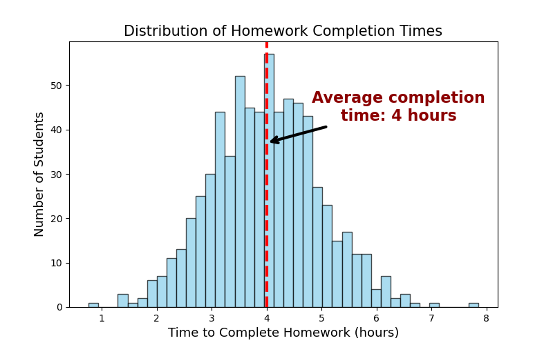
The x-axis represents the time taken to complete the homework, while the y-axis shows the number of students who completed it within that time frame. This graph is called the distribution of the random variable or in this case, the distribution of the time required to complete the first homework. Depending on the students’ preparation and skill set, the distribution may vary. The Figure 2 shows another two scenarios that are relevant to the university homework completion case.
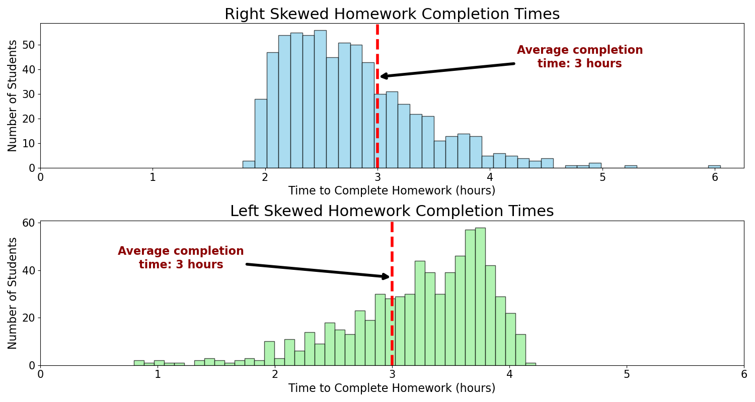
In the first scenario, most students completed the homework within 2 to 3 hours, while a few submitted it much later than the majority. For the second scenario, it took 3 to 4 hours to complete the homework, while few students managed to complete it in 1 to 2 hours. Professors aim to create homework that is challenging enough for most students without being overly difficult. This naturally results in most students completing the work within a similar range of time, with fewer students finishing either very quickly or very slowly. Thus scenario discussed in Figure 1 is preferred and expected. It suggests a normal distribution, also called a Gaussian distribution, one of the most widely used statistical distributions due to its frequent occurrence in real-world data.
What are Statistical Distributions?
A statistical distribution is a key concept in statistics that explains how values are spread across a variable. It represents this spread using a mathematical function or model. Both random variables and their distributions can be categorized as either discrete or continuous. Discrete variables have a finite or countable set of distinct values, while continuous variables can take any value within a given range or interval. The normal distribution is part of the family of continuous distributions.
Normal Distribution
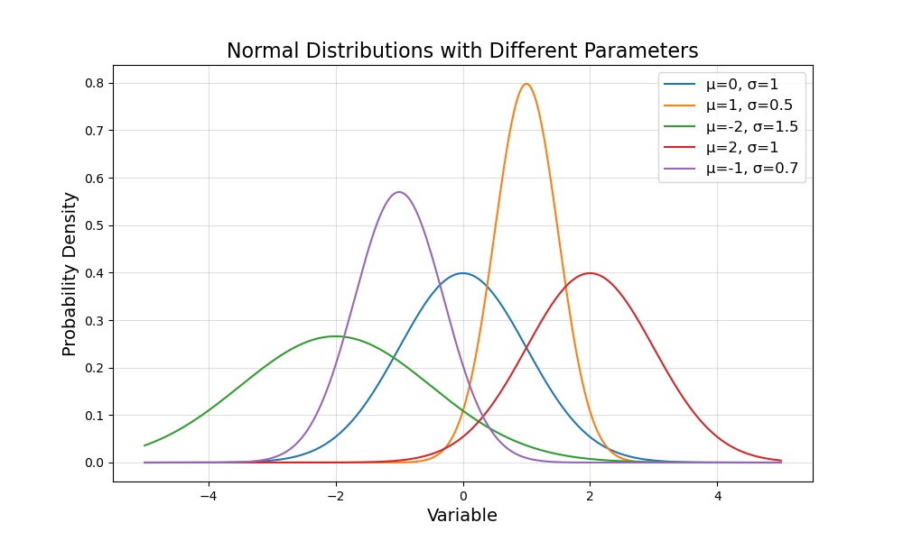
The random variable X = the time required to complete the statistics homework follows a normal distribution with mean 4 hours and standard deviation of 1 hour. Or: \[
N \sim (\mu = 4, \sigma^2=1)
\]
There are two parameters in the normal distribution - \(\mu \text{ and } \sigma\), corresponding to mean and standard deviation respectively. Any combination of the parameters is a new normal distribution. Figure 3 plots different normal distributions.
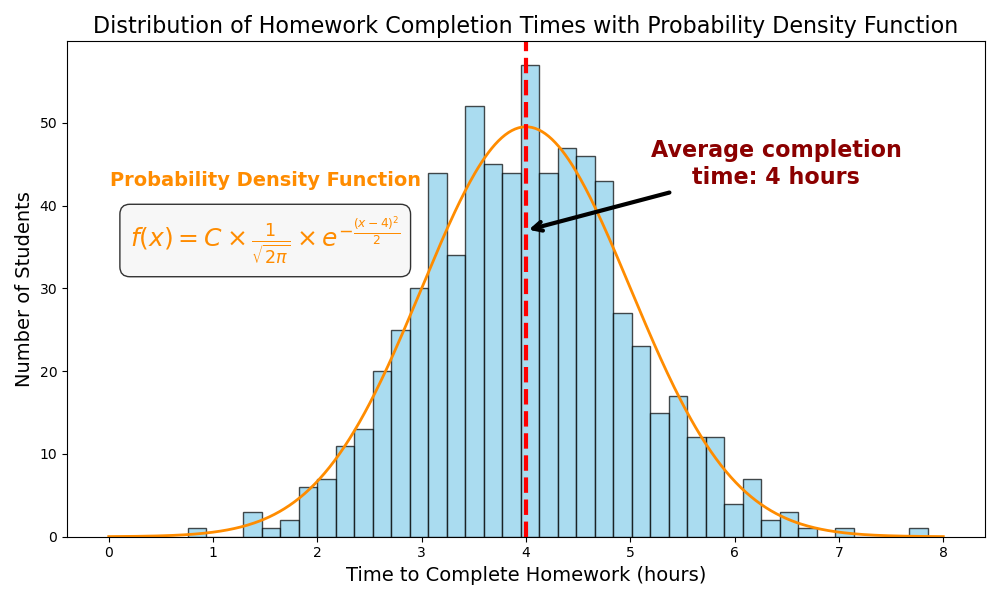
Are these shapes similar to the homework time completion distribution plotted above? Let’s look at Figure 4.
If the data to examine is a bit more noisy, there are more checks to see if the dataset follows a normal distribution or not. For example, QQ-plots, statistical tests like Shapiro-Wilk test or Kolmogorov-Smirnov test.
Probability Density Function is a statistical function that describes the likelihood of a continuous random variable taking on a particular value. The PDF of normal distribution has the following form: \[ f(x) = \frac{1}{\sqrt{2\pi\sigma^2}} \times e^{-\frac{(x - \mu)^2}{2\sigma^2}} \]
In other words, if you plug a number in the function f(x), you will get the density at that specific value. This value represents how concentrated or likely the random variable is to take values near that point, but not the actual probability of the variable being exactly that value (since for continuous distributions, the probability of any specific value is zero). A higher density at a point suggests the random variable is more likely to take values near that point, while a lower density indicates it’s less likely. The scaling factor C is used to convert densities to number of students and match the scale of the plot.
\[ C = \text{Number of students} \times \text{Bin width} \]
Now, when you know that your data follows a normal distribution, lots of opportunities come up:
- Enable parametric tests: Many statistical tests and models assume normality. If your data is normally distributed, you can apply parametric methods, which tend to offer more power and precision compared to non-parametric methods (e.g. Test if the average time to complete the homework is equal to 4 hours for all the students taking statistics using the sample data).
- Prediction: Using the Cumulative Distribution Function (CDF) you can find the probability of students finishing their homework in certain range (e.g. X > 6: What is the probability that a student will finish the homework in more than 6 hours).
- Other: Normal distributions provide additional advantages, such as more reliable confidence intervals, simpler statistical inference, and the ability to use the central limit theorem even with smaller sample sizes.
What is the reason for normal distribution being so popular?
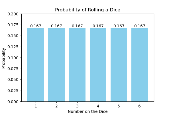
Normal distribution commonly appears in real-world scenarios. One of the main reasons is the important statistical theorem called Central Limit Theorem (CLT). It states that, regardless of the original distribution of data, if you repeatedly take random samples from a population and calculate the mean of each sample, the distribution of those sample means will tend to follow a normal distribution as the sample size increases. Sounds a bit complicated, let’s break down based on an example. The outcomes on the die are 1, 2, 3, 4, 5, or 6, and each number has an equal chance of occurring (\(\frac{1}{6}\)), so the distribution is uniform (see Figure 5).
Now, you want to calculate the average of several rolls of the die. If you roll the die 5 times and calculate the average of those 5 rolls, you will get a number between 1 and 6. If you repeat the process 100 times (rolling the die 100x5 times), you will get 100 averages rolling the die 5 times for each. These averages will likely vary, but if you plot all 100 averages, you’ll notice something interesting (see Figure 6).
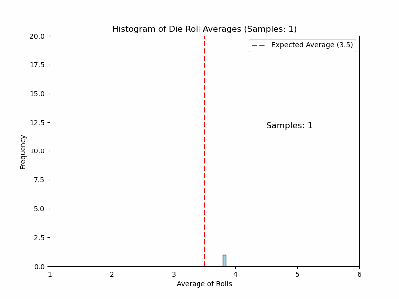
The distribution of those 100 averages will start to look like a normal distribution, even though the original die rolls themselves were uniformly distributed (not normal). The more samples you take, the closer the distribution of averages will be to a normal distribution. What a nice property! Now, as you have a normal distribution for the average, you can run hypothesis tests, get confidence intervals, calculate probabilities, and so on.
Conclusion
The blog explored the normal distribution from a practical, intuitive standpoint. By examining everyday examples like homework completion times and die rolls, the blog showed how the normal distribution naturally emerges in many real-world situations. The key takeaway is that normal distribution isn’t just a theoretical concept but a tool that helps us understand variability and uncertainty in real-world data.
For those struggling to intuitively grasp the normal distribution, remember that it’s simply a way of describing how values spread around a central point. Most values cluster near the mean, with fewer values appearing as you move farther away—just like how most students finish their homework within a certain time frame. Recognizing this pattern in data makes it easier to predict outcomes, perform statistical tests, and make informed decisions.
So, what next? To understand normal distributions deeper, it’s important to explore their use cases in prediction, hypothesis testing, and inference. In prediction, normal distributions help estimate the likelihood of future outcomes, such as the probability of a student finishing homework within a certain time frame. For hypothesis testing, the assumption of normality allows us to apply parametric tests, such as the t-test, to assess whether observed data significantly differs from a hypothesized value. Additionally, normal distributions are essential in statistical inference, as they provide the base for constructing confidence intervals and making reliable conclusions about population parameters from sample data.
Additional Readings
Here are some additional, interesting sources to read and gain better understanding of the material:
- Lyon, A. (2013). Why are Normal Distributions Normal? The British Journal for the Philosophy of Science, 65(3), 621–649. https://doi.org/10.1093/bjps/axs046
- Bryc, W. (1995). Normal distributions. In: The Normal Distribution. Lecture Notes in Statistics, vol 100. Springer, New York, NY. https://doi.org/10.1007/978-1-4612-2560-7_3
End
Thank you for taking the time to read this blog! I hope it has provided you with a clearer understanding of the significance of normal distributions and how they appear in real-world scenarios.